Gaussian Mixture Models in PyTorch
Update: Revised for PyTorch 0.4 on Oct 28, 2018
Introduction
Mixture models allow rich probability distributions to be represented as a combination of simpler “component” distributions. For example, consider the mixture of 1-dimensional gaussians in the image below:
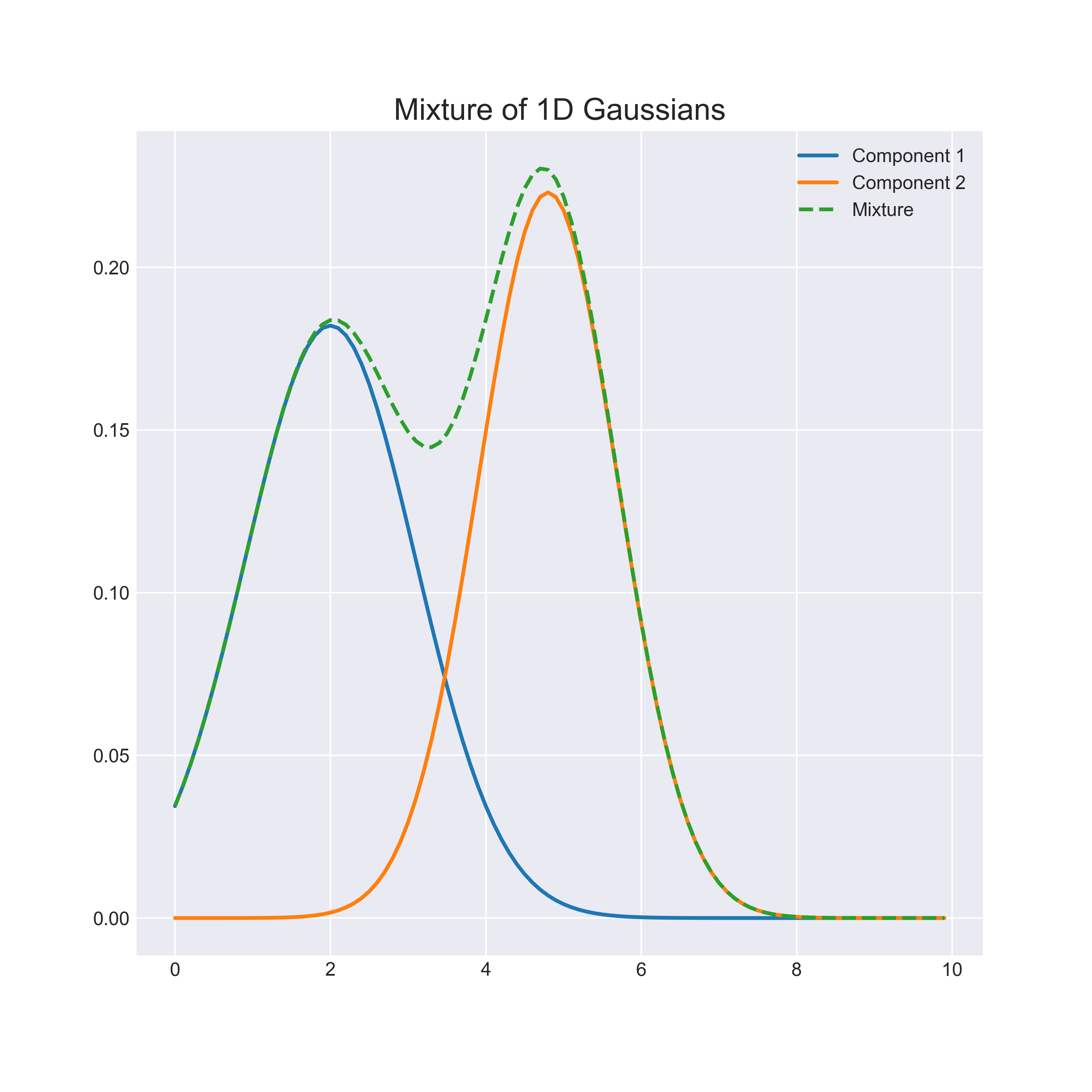
While the representational capacity of a single gaussian is limited, a mixture is capable of approximating any distribution with an accuracy proportional to the number of components2.
In practice mixture models are used for a variety of statistical learning problems such as classification, image segmentation and clustering. My own interest stems from their role as an important precursor to more advanced generative models. For example, variational autoencoders provide a framework for learning mixture distributions with an infinite number of components and can model complex high dimensional data such as images.
In this blog I will offer a brief introduction to the gaussian mixture model and implement it in PyTorch. The full code will be available on my github.
The Gaussian Mixture Model
A gaussian mixture model with \(K\) components takes the form1:
\[p(x) = \sum_{k=1}^{K}p(x|z=k)p(z=k)\]where \(z\) is a categorical latent variable indicating the component identity. For brevity we will denote the prior \(\pi_k := p(z=k)\) . The likelihood term for the kth component is the parameterised gaussian:
\[p(x|z=k)\sim\mathcal{N}(\mu_k, \Sigma_k)\]Our goal is to learn the means \(\mu_k\) , covariances \(\Sigma_k\) and priors \(\pi_k\) using an iterative procedure called expectation maximisation (EM).
The basic EM algorithm has three steps:
- Randomly initialise the parameters of the component distributions.
- Estimate the probability of each data point under the component parameters.
- Recalculate the parameters based on the estimated probabilities. Repeat Step 2.
Convergence is reached when the total likelihood of the data under the model stops decreasing.
Synthetic Data
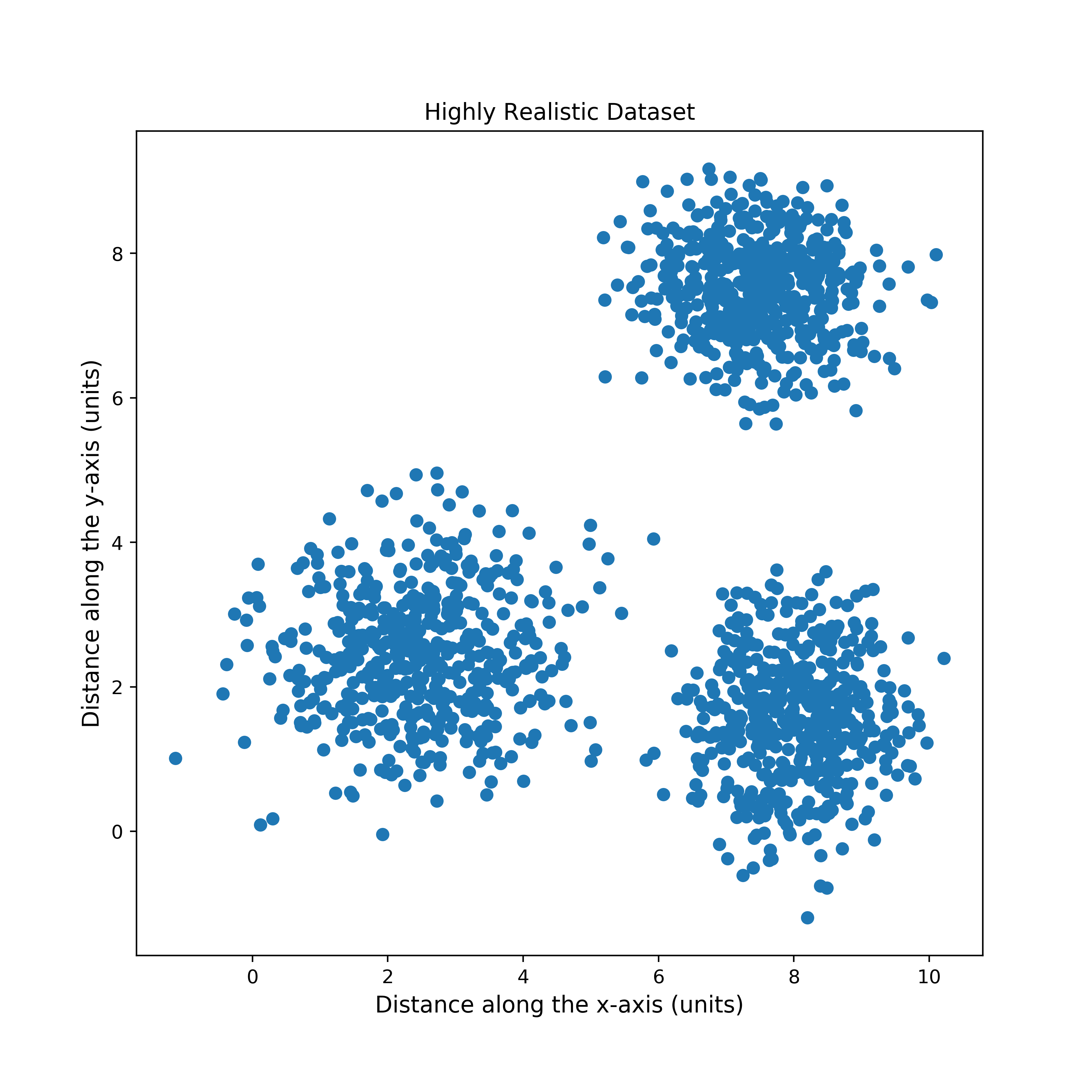
In order to quickly test my implementation, I created a synthetic dataset of points sampled from three 2-dimensional gaussians, as follows:
def sample(mu, var, nb_samples=500):
    """
    :param mu: torch.Tensor (features)
    :param var: torch.Tensor (features) (note: zero covariance)
    :return: torch.Tensor (nb_samples, features)
    """
    out = []
    for i in range(nb_samples):
        out += [
            torch.normal(mu, var.sqrt())
        ]
    return torch.stack(out, dim=0)
Initialising the Parameters
For the sake of simplicity, I just randomly select K points from my dataset to
act as initial means. I use a fixed initial variance and a uniform prior.
def initialize(data, K, var=1):
  """
  :param data: design matrix (examples, features)
  :param K: number of gaussians
  :param var: initial variance
  """
  # choose k points from data to initialize means
  m = data.size(0)
  idxs = torch.from_numpy(np.random.choice(m, k, replace=False))
  mu = data[idxs]

  # uniform sampling for means and variances
  var = torch.Tensor(k, d).fill_(var)

  # uniform prior
  pi = torch.empty(k).fill_(1. / k)

  return mu, var, pi
The Multivariate Gaussian
Step 2. of the EM algorithm requires us to compute the relative likelihood of each data point under each component. The p.d.f of the multivariate gaussian is
\[p(x;\mu, \sigma)=\frac{1}{\sqrt{2\pi|\Sigma|} }\exp\left(-\frac{1}{2}(x-\mu)^T\Sigma^{-1}(x-\mu)\right)\]By only considering diagonal covariance matrices \(I\sigma^2 = \Sigma\) , we can greatly simplify the computation (at the loss of some flexibility):
\[|\Sigma| = \prod_{j=1}^{N}\sigma_{j}^{2}\]Instead of computing the matrix inverse we can simply invert the variances.
\[Tr(\Sigma^{-1}) = \left[\sigma_1^{-2}, ..., \sigma_N^{-2}\right]\]And lastly, the exponent simplifies to,
\[-\frac{1}{2}\left(\left(x-\mu\right)\odot\left(x-\mu\right)\right)^{T}\sigma^{-2}\]where \(\odot\) represents element-wise multiplication and \(\sigma^{-2}\) is our vector of inverse variances.
It is worth taking a minute to reflect on the form of the exponent in the last equation. Because there is no linear dependence between the dimensions, the computation reduces to calculating a gaussian p.d.f for each dimension independently and then taking their product (or sum in the log domain).
Calculating Likelihoods
In high dimensions the likelihood calculation can suffer from numerical underflow. It is therefore typical to work with the log p.d.f instead (i.e. the exponent we derived above, plus the constant normalisation term). Note that we could use the in-built PyTorch distributions package for this, however for transparency here is my own functional implementation:
log_norm_constant = -0.5 * np.log(2 * np.pi)

def log_gaussian(x, mean=0, logvar=0.):
  """
  Returns the density of x under the supplied gaussian. Defaults to
  standard gaussian N(0, I)
  :param x: (*) torch.Tensor
  :param mean: float or torch.FloatTensor with dimensions (*)
  :param logvar: float or torch.FloatTensor with dimensions (*)
  :return: (*) elementwise log density
  """
  if type(logvar) == 'float':
      logvar = x.new(1).fill_(logvar)

  a = (x - mean) ** 2
  log_p = -0.5 * (logvar + a / logvar.exp())
  log_p = log_p + log_norm_constant

  return log_p
To compute the likelihood of every point under every gaussian in parallel, we can exploit tensor broadcasting as follows:
def get_likelihoods(X, mu, logvar, log=True):
  """
  :param X: design matrix (examples, features)
  :param mu: the component means (K, features)
  :param logvar: the component log-variances (K, features)
  :param log: return value in log domain?
      Note: exponentiating can be unstable in high dimensions.
  :return likelihoods: (K, examples)
  """

  # get feature-wise log-likelihoods (K, examples, features)
  log_likelihoods = log_gaussian(
      X[None, :, :], # (1, examples, features)
      mu[:, None, :], # (K, 1, features)
      logvar[:, None, :] # (K, 1, features)
  )

  # sum over the feature dimension
  log_likelihoods = log_likelihoods.sum(-1)

  if not log:
      log_likelihoods.exp_()

  return log_likelihoods
Computing Posteriors
In order to recompute the parameters we apply Bayes rule to likelihoods as follows:
\[p(z|x)=\frac{p(x|z)p(z)}{\sum_{k}^{K}p(x|z=k)p(z=k)}\]The resulting values are sometimes referred to as the “membership weights”, as they \(z\) can explain the observation \(x\). Since our likelihoods are in the log-domain, we exploit the logsumexp trick for stability.
def get_posteriors(log_likelihoods):
  """
  Calculate the the posterior probabilities log p(z|x), assuming a uniform prior over
  components.
  :param likelihoods: the relative likelihood p(x|z), of each data point under each mode (K, examples)
  :return: the log posterior p(z|x) (K, examples)
  """
  posteriors = log_likelihoods - logsumexp(log_likelihoods, dim=0, keepdim=True)
  return posteriors
Parameter Update
Using the membership weights, the parameter update proceeds in three steps:
- Set new mean for each component to a weighted average of the data points.
- Set new covariance matrix as weighted combination of covariances for each data point.
- Set new prior, as the normalised sum of the membership weights.
def get_parameters(X, log_posteriors, eps=1e-6, min_var=1e-6):
  """
  :param X: design matrix (examples, features)
  :param log_posteriors: the log posterior probabilities p(z|x) (K, examples)
  :returns mu, var, pi: (K, features) , (K, features) , (K)
  """

  posteriors = log_posteriors.exp()

  # compute `N_k` the proxy "number of points" assigned to each distribution.
  K = posteriors.size(0)
  N_k = torch.sum(posteriors, dim=1) # (K)
  N_k = N_k.view(K, 1, 1)

  # get the means by taking the weighted combination of points
  # (K, 1, examples) @ (1, examples, features) -> (K, 1, features)
  mu = posteriors[:, None] @ X[None,]
  mu = mu / (N_k + eps)

  # compute the diagonal covar. matrix, by taking a weighted combination of
  # the each point's square distance from the mean
  A = X - mu
  var = posteriors[:, None] @ (A ** 2) # (K, 1, features)
  var = var / (N_k + eps)
  logvar = torch.clamp(var, min=min_var).log()

  # recompute the mixing probabilities
  m = X.size(1) # nb. of training examples
  pi = N_k / N_k.sum()

  return mu.squeeze(1), logvar.squeeze(1), pi.squeeze()
Results
Apart from some simple training logic, that is the bulk of the algorithm! Here is a visualisation of EM fitting three components to the synthetic data I generated earlier:
Thanks for Reading!
If you found this post interesting or informative, have questions or would like to offer feedback or corrections feel free to get in touch at my email or on twitter. Also stay tuned for my upcoming post on Variational Autoencoders!
References
For a more rigorous treatment of the EM algorithm see [1].
- Bishop, C. (2006). Pattern Recognition and Machine Learning. Ch9.
- Bengio, Y., Goodfellow, I. (2016). Deep Learning.