Diffusion Models as a kind of VAE

\[\require{cancel}\]

Introduction

Recently I have been studying a class of generative models known as diffusion probabilistic models. These models were proposed by Sohl-Dickstein et al. in 2015 [1], however they first caught my attention last year when Ho et al. released “Denoising Diffusion Probabilistic Models” [2]. Building on [1], Ho et al. showed that a model trained with a stable variational objective could match or surpass GANs on image generation.

Since the release of DDPM there has been a wave of renewed interest in diffusion models. New works have extended their success to the domain of audio modelling [8][16], text-to-speech [9], and multivariate time-series forecasting [10]. Furthermore, as shown by Ho et al. [2], these models exhibit close connections with score-based models [11], and the two perspectives were recently unified under the framework of stochastic differential equations [4].

As a generative model, diffusion models have a number of unique and interesting properties. For example, trained models are able to perform inpainting [1] and zero-shot denoising [8] without being explicitly designed for these tasks. Furthermore, the variational bound used in DDPM highlights further connections to variational autoencoders and neural compression.

In this blog I want to explore diffusion models as they are presented in Sohl-Dickstein et al. [1], and Ho et al. [2]. When I was working through these derivations, I found it useful to conceptualise these models in terms of their relationship to VAEs [3]. For this reason, I want to work up from a simple VAE derivation, through to hierarchical extensions, and finally the deep generative model presented in [1] and [2]. I will conclude with some thoughts on the relationship between the two models, and some possible ideas for further research.

I have also released a PyTorch implementation of my code.

Variational Autoencoders

I want to begin with a quick refresher of variational autoencoders [3]. If this is all feels familiar to you, feel free to skip ahead!

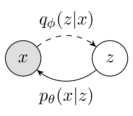
Consider the following generative model,

\[p_{\theta}(x) = \int_{z}p_{\theta}(x|z)p_{\theta}(z)\]

Where \(x\) is the data we would like to model and \(z\) is a latent variable. In general, the form of the prior \(p_{\theta}(z)\) and observation model \(p_{\theta}(x|z)\) will depend on the data we are trying to model. For now lets assume \(p(z) := \mathcal{N}(0, I)\) and \(p_{\theta}(x|z)\) as a factorised gaussian, whose parameters \(\mu_{\theta}(z)\) and \(\sigma_{\theta}(z)\) we will predict with a neural network.

Of course, for most problems we do not have access to the true distribution \(p(x)\), and would like to fit our model to some empirically observed subset \(\hat{p}(x)\). Naively, we could try to estimate the model parameters \(\theta\) with MLE, using monte-carlo sampling to approximate the integral over \(z\).

\[\theta^{*} = \underset{\theta}{\text{argmax}} \text{ } \mathbb{E}_{x \sim \hat{p}(x) \text{, } z \sim p(z)} \left[ \text{log } p_{\theta}(x|z; \theta) \right]\]

However, it is well known that this approach does not scale to high dimensions of \(z\) [5]. Intuitively, the likelihood of a random latent code \(z \sim p(z)\) corresponding to any particular data point is extremely small (especially in high dimensions!).

The VAE solves this problem by sampling \(z\) from a new distribution \(q_{\phi}(z|x)\), which is jointly optimised with the generative model. This focuses the optimisation on regions of high probability (i.e. latent codes that are likely to have generated \(x\)).

This can be derived as follows:

\[p(x) = \int_{z} p_{\theta}(x|z)p(z) \\ p(x) = \int q_{\phi}(z|x) \frac{p_{\theta}(x|z)p(z)}{q_{\phi}(z|x)}\\ \text{log }p(x) = \text{log } \mathbb{E}_{z \sim q_{\phi}(z|x)} \left[ \frac{p_{\theta}(x|z)p(z)}{q_{\phi}(z|x)} \right]\\ \text{log }p(x) \geq \mathbb{E}_{z \sim q_{\phi}(z|x)} \left[ \text{log } \frac{p_{\theta}(x|z)p(z)}{q_{\phi}(z|x)} \right]\]

The final step follows from Jensen’s inequality and the fact that log is a concave function. The right-hand side of this inequality is the evidence lower-bound (ELBO), sometimes denoted \(\mathcal{L}(\theta, \phi)\). The ELBO provides a joint optimisation objective, which simultaneously updates the variational posterior \(q_{\phi}(z|x)\) and likelihood model \(p_{\theta}(x|z)\).

To optimise the ELBO we have to obtain gradients for \(\phi\) through a stochastic sampling operation \(z \sim q_{\phi}(z|x)\). Kingma and Welling famously solved this with a “reparameterization trick”, which defines the sampling process as a combination of a deterministic data-dependent function and data-independent noise [3].

Figure 1 - Graphical Model for VAE

So much has been written about VAEs that I am barely scratching the surface here. For those interested to learn more, see the section on further reading.

Hierarchical Variational Autoencoders

Having defined a VAE with a single stochastic layer, it is straightforward to derive hierarchical extensions. Consider a VAE with two latent variables \(z_1\) and \(z_2\). We begin by considering the joint distribution \(p(x, z_1, z_2)\) and marginalising out the latent variables:

\[p(x) = \int_{z_1} \int_{z_2} p_{\theta}(x, z_1, z_2) dz_1, dz_2\]

We introduce a variational approximation to the true posterior,

\[p(x) = \int \int q_{\phi}(z_1, z_2|x) \frac{p_{\theta}(x, z_1, z_2)}{q_{\phi}(z_1, z_2|x)}\\ p(x) = \mathbb{E}_{z_1 ,z_2 \sim q_{\phi}(z_1, z_2|x)} \left[ \frac{p_{\theta}(x, z_1, z_2)}{q_{\phi}(z_1, z_2|x)} \right]\]

Taking the log and applying Jensen’s rule:

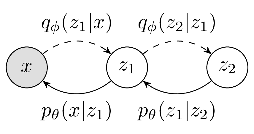
\[\text{log } p(x) \geq \mathbb{E}_{z_1 ,z_2 \sim q_{\phi}(z_1, z_2|x)} \left[ \text{log } \frac{p_{\theta}(x, z_1, z_2)}{q_{\phi}(z_1, z_2|x)} \right]\]

Notice that I have written these expressions in terms of the joint distributions \(p_{\theta}(x, z_1, z_2)\) and \(q_{\phi}(z_1, z_2|x)\). I have done this to emphasise the fact that we are free to factorise the inference and generative models as we see fit. In practice, some factorisations are more suitable than others (as shown in [7]). For now lets consider the model in Figure 2.

Figure 2 - A Hierarchical VAE

For the generative pathway we have,

\[p(x,z_1,z_2) = p(x|z_1)p(z_1|z_2)p(z_2)\]

and the inference model,

\[q(z_1,z_2|x) = q(z_1|x)q(z_2|z_1)\]

Substituting these factorizations into the ELBO, we get:

\[\mathcal{L}(\theta, \phi) = \mathbb{E}_{q(z_1, z_2|x)} \left[ \text{log }p(x|z_1) - \text{log }q(z_1|x) + \text{log }p(z_1|z_2) - \text{log }q(z_2 | z_1) + \text{log }p(z_2) \right]\\\]

This can be alternatively written as a “reconstruction term”, and the KL divergence between each inference layer and its corresponding prior:

\[= \mathbb{E}_{q(z_1|z_2)} \left[ \text{log }p(x|z_1) \right] - D_{KL} \left( q(z_1|x) \mathrel{\Vert} p(z_1|x) \right) - D_{KL} \left( q(z_2|z_1) \mathrel{\Vert} p(z_2) \right)\]

Diffusion Probabilistic Models

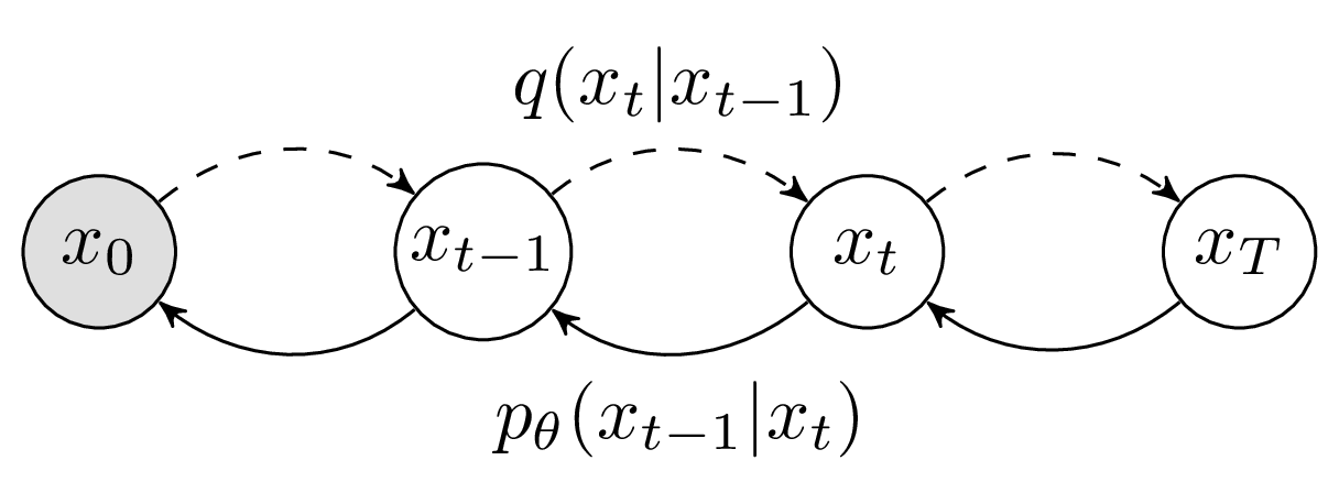
Now consider the model in Figure 3. We have sequence of \(T\) variables, where \(x_0 \sim p(x)\) is our observed data and \(x_{1:T}\) are latent variables.

Figure 3 - Diffusion Probabilistic Model

The lower bound for this model should look quite familiar by now (negated, for consistency with Ho et al. [2]):

\[- \mathcal{L} = \mathbb{E}_{q} \left[ -\text{log }p(x_T) - \sum_{t \geq 1}^{T} \text{log } \frac{p_{\theta}(x_{t-1}|x_t)}{q(x_t|x_{t-1})} \right]\]

In fact, we can think of diffusion models as a specific realisation of a hierarchical VAE. What sets them apart is a unique inference model, which contains no learnable parameters and is constructed so that the final latent distribution \(q(x_T)\) converges to a standard gaussian. This “forward process” model is defined as follows:

\[q(x_t|x_{t-1}) = \mathcal{N}(x_T\mathrel{;} x_{t-1}\sqrt{1 - \beta_{t}}, \beta_{t}I)\]

The variables \(\beta_1 \dots \beta_{T}\) define a fixed variance schedule, chosen such that \(q(x_T|x_0) \approx \mathcal{N}(0, I)\). The forward process is illustrated below, transforming samples from the 2d swiss roll distribution into gaussian noise:

A nice property of the forward process is that we can directly sample from any timestep:

\[\alpha_t := 1-\beta_t\\ \bar{\alpha}_t := \prod_{s=1}^{t} \alpha_s \\ q(x_t|x_0) = \mathcal{N}\left(\sqrt{\bar{\alpha}_t}x_0, (1-\bar{\alpha}_t)I \right)\]

One consequence of this, is that we can draw random samples \(t ~ \sim \{1 \dots T \}\) as part of training procedure, optimising a random set of conditionals \(p_{\theta} ( x_{t-1} | x_t )\) with each minibatch. In other words, we do not have to do a complete pass of the forward and reverse processes on each step of training.

Another consequence, is that we can make additional manipulations to the lower-bound to reduce the variance. This proceeeds by observing the following result (from bayes rule):

\[q(x_t|x_{t-1}) = \frac{q(x_{t-1}|x_t)q(x_t)}{q(x_{t-1})}\]

The terms \(q(x_t)\) and \(q(x_{t-1})\) are intractable to compute, as they would require marginalising over all data points. However, due to the markov propety of the forward process we have:

\[q(x_t|x_{t-1}) = q(x_t|x_{t-1},x_0)\]

Therefore, by conditioning all terms on \(x_0\) we arrive at the following expression.

\[q(x_t|x_{t-1}) = \frac{q(x_{t-1}|x_t,x_0)q(x_t|x_0)}{q(x_{t-1}|x_0)} \tag{1}\]

We now have an equation with one unknown \(q(x_{t-1}|x_t,x_0)\). This is referred to as the “forward process posterior”, and we will return to it shortly. First, lets continue our work on the ELBO.

Separating the contribution from the first term in the sum:

\[L = \mathbb{E}_{q} \left[ -\text{log }p(x_T) - \text{log } \frac{p_{\theta}(x_0|x_1)}{q(x_1|x_0)} - \sum_{t \gt 1}^{T} \text{log } \frac{p_{\theta}(x_{t-1}|x_t)}{q(x_t|x_{t-1})} \right] \tag{2}\]

Substituting (1) into (2),

\[\mathbb{E}_{q} \left[ -\text{log }p(x_T) - \text{log } \frac{p_{\theta}(x_0|x_1)}{q(x_1|x_0)} - \sum_{t \gt 1}^{T} \left( \text{log } \frac{p_{\theta}(x_{t-1}|x_t)}{q(x_{t-1}|x_t,x_0)} + \text{log } \frac{q(x_{t-1}|x_0)}{q(x_t|x_0)} \right) \right]\]

Notice what happens what happens to the conditionals \(q(x_t|x_0)\) when we expand the sum:

\[\cancel{\text{log }q(x_1|x_0)} - \cancel{\text{log }q(x_1|x_0)} + \dots + \text{log }q(x_T|x_0)\]

These cancellations lead to the following negative bound:

\[L := \mathbb{E}_{q} \left[ \underbrace{-\text{log }p(x_T) + \text{log }q(x_T|x_0)}_{L_T} - \underbrace{\text{log } p_{\theta}(x_0|x_1)}_{L_0} - \underbrace{\sum_{t \gt 1}^{T} \text{log } \frac{p_{\theta}(x_{t-1}|x_t)}{q(x_{t-1}|x_t,x_0)}}_{L_{t-1}} \right]\]

\(L_T\) has no parameters, and simply measures the effectiveness of the forward process in producing a standard gaussian. The summands in \(L_{t-1}\) are KL divergences between gaussians, which can be calculated in closed-form (as opposed to using high variance monte-carlo estimates). Lastly, \(L_0\) is the familiar reconstruction term.

Denoising Diffusion Probabilistic Models

So far our derivation matches with the original Sohl-Dickstein et al. paper [1], with notation borrowed from [2] for consistency. In DDPM, Ho et al. propose a specific parameterization of the generative model, which simplifies the training and connects it to score based modelling.

We start by noting the form of the forward process posterior. This result can be derived from bayes rule, substituting the known gaussian conditionals into equation (1). For those interested, a detailed derivation is presented by Kong et al. [8] (Appendix A).

\[q(x_{t-1}|x_t,x_0) = \mathcal{N}(x_{t-1};\tilde{\mu}(x_t,x_0),\tilde{\beta}_t I)\\ \tilde{\mu}_t(x_t,x_0) = \frac{ \sqrt{\bar{\alpha}_{t-1}} \beta_{t} }{1 - \bar{\alpha}_t} x_0 + \frac{ \sqrt{\alpha_t} (1 - \bar{\alpha}_{t-1}) }{1 - \bar{\alpha}_t} x_t \tag{3} \\ \tilde{\beta}_t = \frac{ 1 - \bar{\alpha}_{t-1} }{1 - \bar{\alpha}_t } \beta_t\]

The corresponding reverse process distributions are defined as:

\[p_{\theta}(x_{t-1}|x_t) = \mathcal{N}(x_{t-1}; \mu_{\theta}(x_t, t), \sigma_{t}^2 I)\]

The variance \(\sigma_{t}^2\) is a time-dependent constant (either \(\beta_t\) or \(\tilde{\beta}_t)\). The mean \(\mu_{\theta}(x_t, t)\) is a neural network, which takes as input \(x_t\). In order to share parameters between timesteps, the conditioning variable \(t\) is introduced in the form of positional embeddings [12].

With these definitions, the KL divergence terms in \(L_{t-1}\) reduce to the following mean-square error:

\[L_{t-1} = \mathbb{E}_{t,x_t,x0} \left[ \frac{1}{2\sigma_t^2} \lVert \tilde{\mu}_t(x_t,x_0) - \mu_{\theta}(x_t, t) \rVert \right] + C \tag{4}\]

This objective is suitable for optimisation, however Ho et al. continue expanding to arrive at an alternative denoising objective. Note that forward process samples \(x_t\) can be written as a function of \(x_0\) and some noise \(\epsilon \sim \mathcal{N}(0, I)\).

\[x_t(x_0, \epsilon) = \sqrt{\bar{\alpha}_t}x_0 + \sqrt{1 - \bar{\alpha}_t} \epsilon \tag{5}\]

Conversely, for a given sample \(x_t(x_0, \epsilon)\) we can express \(x_0\) as,

\[x_0 = \frac{x_t(x_0, \epsilon) - \sqrt{1 - \bar{\alpha}_t} \epsilon}{\sqrt{\bar{\alpha}_t}} \tag{6}\]

At this point, Ho et al. rewrite the forward process posterior mean (3) in terms of \(x_t(x_0, \epsilon)\), by evaluating:

\[\tilde{\mu}_t \left( x_t(x_0, \epsilon), \frac{1}{\sqrt{\bar{\alpha}_t}} \left( x_t(x_0, \epsilon) - \sqrt{1 - \bar{\alpha}_t} \epsilon \right) \right)\]

This expands to,

\[= \frac{ \beta_{t} \sqrt{\bar{\alpha}_{t-1}} (x_t - \epsilon \sqrt{1 - \bar{\alpha}_t}) }{\sqrt{\bar{\alpha}_t}(1 - \bar{\alpha}_t)} + \frac{ \sqrt{\alpha_t} (1 - \bar{\alpha}_{t-1}) }{1 - \bar{\alpha}_t} x_t\\ = \left( \frac{ \beta_{t} \sqrt{\bar{\alpha}_{t-1}} }{ \sqrt{\bar{\alpha}_t}(1 - \bar{\alpha}_t) } + \frac{ \sqrt{\alpha_t} (1 - \bar{\alpha}_{t-1}) }{1 - \bar{\alpha}_t} \right) x_t - \frac{\beta_t \sqrt{\bar{\alpha}_{t-1}} \sqrt{1 - \bar{\alpha}_{t}}}{ \sqrt{\bar{\alpha}_t}(1 - \bar{\alpha}_t) } \epsilon\]

With a bit of manipulation this can be drastically simplified. Lets deal with the coeffient of \(x_t\) first, using the fact that \(\bar{\alpha}_t = \bar{\alpha}_{t-1} \alpha_t\) and \(\beta_t = 1 - \alpha_t\):

\[= \left( \frac{ \beta_{t} \sqrt{\bar{\alpha}_{t-1}} }{ \sqrt{\bar{\alpha}_t}(1 - \bar{\alpha}_t) } + \frac{ \sqrt{\alpha_t} (1 - \bar{\alpha}_{t-1}) }{1 - \bar{\alpha}_t} \right) \cdot \frac{ \sqrt{\alpha_t} }{ \sqrt{\alpha_t} } \\ = \frac{ \beta_{t} \sqrt{\bar{\alpha}_{t}} }{ \sqrt{\alpha_t}\sqrt{\bar{\alpha}_t}(1 - \bar{\alpha}_t) } + \frac{ \alpha_t (1 - \bar{\alpha}_{t-1}) }{\sqrt{\alpha_t}(1 - \bar{\alpha}_t)} \\ = \frac{1}{\sqrt{\alpha_t}} \cdot \frac{\beta_t + \alpha_t(1 - \bar{\alpha}_{t-1})}{1 - \bar{\alpha}_t}\\ = \frac{1}{\sqrt{\alpha_t}} \cdot \frac{1 - \alpha_t + \alpha_t - \alpha_t \bar{\alpha}_{t-1}}{1 - \bar{\alpha}_t}\\ = \frac{1}{\sqrt{\alpha_t}}\]

The coefficient of \(\epsilon\) simplifies to,

\[= - \frac{\beta_t}{\sqrt{\alpha_t} \sqrt{1 - \bar{\alpha}_t}}\]

Now we can rewrite (4) as follows,

\[L_{t-1} - C = \mathbb{E}_{x_0,\epsilon,t} \left[ \frac{1}{2\sigma_t^2} \left\lVert \frac{1}{\sqrt{\alpha_t}} \cdot \left( x_t(x_0, \epsilon) - \frac{\beta_t}{\sqrt{1 - \bar{\alpha}_t}} \epsilon \right) - \mu_{\theta}(x_t(x_0, \epsilon), t) \right\rVert \right] \tag{7}\]

From (7), we observe that the loss is minimised when \(\mu_{\theta}\) predicts,

\[\frac{1}{\sqrt{\alpha_t}} \cdot \left( x_t(x_0, \epsilon) - \frac{\beta_t}{\sqrt{1 - \bar{\alpha}_t}} \right)\]

In other words, we are providing the model with \(x_t, t\) and asking it to predict some affine transformation of \(x_t\). This affine transform is a combination of time-dependent constants, and a single free parameter \(\epsilon\). This motivates an alternative parameterisation, where the neural net is only responsible for predicting the noise \(\epsilon\).

\[\mu_{\theta}(x_t, t) = \frac{1}{\sqrt{\alpha_t}} \cdot \left( x_t(x_0, \epsilon) - \frac{\beta_t}{\sqrt{1 - \bar{\alpha}_t}} \epsilon_{\theta}(x_t(x_0, \epsilon), t) \right) \tag{8}\]

Substituting (8) into (7),

\[= \mathbb{E}_{x_0,\epsilon,t} \left[ \frac{1}{2\sigma_t^2} \left\lVert \frac{\beta_t}{ \sqrt{\alpha_t} \sqrt{1 - \bar{\alpha}_t} } \cdot \left( \epsilon - \epsilon_{\theta}(x_t(x_0, \epsilon), t) \right) \right\rVert \right]\\\] \[= \mathbb{E}_{x_0,\epsilon,t} \left[ \frac{\beta_t^2}{2\sigma_t^2 \alpha_t (1 - \bar{\alpha}_t)} \left\lVert \epsilon - \epsilon_{\theta}(x_t(x_0, \epsilon), t) \right\rVert \right] \tag{9}\]

Finally Ho et al. note that omitting the term \(\frac{\beta_t^2}{2\sigma_t^2 \alpha_t (1 - \bar{\alpha}_t)}\) leads to weighted variant of the lower bound, which (aside from being simpler) leads to better empirical results.

\[= \mathbb{E}_{x_0,\epsilon,t} \left[ \left\lVert \epsilon - \epsilon_{\theta}(x_t(x_0, \epsilon), t) \right\rVert \right] \tag{10}\]

DDPM Interpretation

On its own the DDPM derivation can seem a bit daunting. Let’s summarise:

The training objective in Equation (10) corresponds to a single layer of the variational bound.
We sample a data point \(x_0 \sim p(x)\), a random timestep \(t\) and some noise \(\epsilon \sim \mathcal{N}(0, I)\)
Based on the properties of the forward process, we can compute \(x_t(x_0, \epsilon)\), which represents a sample from \(q(x_t|x_0)\).
The forward process posterior \(q(x_{t-1}|x_t,x_0)\) has a closed-form distribution, which we compute based on knowing \(x_0\) and \(x_t\).
We want to minimise the KL divergence between each generative layer \(p_{\theta}(x_{t-1}|x_t)\) and the corresponding forward process posterior.
By analysing the bound we see that minimising this divergence is equivalent to predicting the noise \(\epsilon\) that is required to invert the forward process.

Is DDPM a kind of VAE?

Okay, so while it technically optimises a variational bound, the DDPM model looks quite different from the VAE presented by Kingma. Some of you are probably thinking: Is it really fair to claim this is a kind of VAE?

I suspect this this is largely a matter of semantics. However, we can say that DDPM is similar to VAE in the following respects:

We have a generative model (the reverse process) that involves sampling some latent variable and transforming it into data with a neural network
We have a corresponding inference model (the forward process), which transforms data into a series of latent representations.
The training objective is a lower bound on the data likelihood, which can be derived in a similar fashion to the VAE.

We also have the following key differences:

The inference model or ‘forward process’ in DDPM has no learned parameters
The forward process in DDPM progressively destroys all information about the input, such that the final distribution \(q(x_T|x_0)\) is a standard gaussian by construction. This is typically not true with VAEs (we want z to contain some information about x !)
In DDPM the dimensionality of each latent must match the data. In VAEs we can reduce dimensionality.
In DDPM, each generative layer shares the same neural network parameters. This is not typical for VAEs, however it should be possible in theory (I am not sure if it has been explored).

I think it is interesting to think about how the overlap between VAE and DDPM might inspire future research directions. For example, there have been countless proposed variations and improvements to the VAE, including all kinds of flexible posterior and prior distributions [7][17], decoders [18], constrained optimisation techniques [20], and connections to information theory and compression [19]. Perhaps some of these insights from the VAE literature could be translatable to DDPM (and vice versa).

Open Questions

Studying DDPM has raised a lot of questions for me. I thought I would share just a couple, in case they are of any interest to others!

Can we do a multi-scale DDPM model, which progressively factorises out latent dimensions, similar to the multi-scale architecture in RealNVP [14]? Perhaps the forward process could go at different rates for different latent subsets.
Can we fit a diffusion model in the latent space of an autoencoder, as a means to:
- a) sample from a deterministic autoencoder, as was done with GMMs in [13].
- b) learn regions of the latent space that correspond to certain known attributes [15]
Can we use more flexible distributions for the forward process? For example, it was noted in [4] that sampling \(q(x_t|x_0)\) requires solving “Kolmogorov’s forward equation” for the chosen process. However, perhaps for some flexible \(q_{\phi}(x_t|x_{t-1})\) we could sample from a (jointly learned) approximation \(q_{\phi}(x_t|x_0)\) ?

As another way to state 3., perhaps there is some middle ground between diffusion models and VAE. For example, we could retain the DDPM property of sharing parameters between each generative layer, and training them independently, while also utilising a learned inference model.

Conclusion

If you’ve made it this far, I hope that you have found these notes helpful! There is so much more that can be said about diffusion models, and in fact I still have a great deal to learn myself. For example, I have not even touched on the connection to score-based models or SDEs. However, there is a great blog by Yang Song that goes into detail about these connections.

A lot of the derivations I have presented can be found in the original papers, and I encourage you to go through them yourself! I hope that by expanding on them step-by-step I have made them a bit easier to follow along with and get some intuition. If you have any questions, or just want to discuss diffusion models further, please feel free to reach out by email or on twitter. Also feel free to check out the corresponding code.